Data Analysis

Overview

This guide will take you through all the steps you need to handle your Gorilla data.

Find out about file formats, how to understand your data, and exactly what each column in your data file means.

Then find out to process and analyse your data in Microsoft Excel or RStudio with our handy walkthroughs and tutorials.

If you're using mousetracking or eyetracking in the older Task Builder 1, we have specific guides for analysing these using RStudio:

• Mousetracking data analysis
• Eyetracking data analysis

Data Format

Data files

It's good practice (and in compliance with the British Psychological Society requirements) to keep performance data, demographic data, and identifying data separate, which is why we give you a separate file for each node in your experiment tree.

You can combine data from tasks and questionnaires into a single file in external software by matching the data up by the participants IDs, which we'll show you how to do throughout these guides in both RStudio and Excel.

You can also see an example of how to do this with data from a real experiment, and download the relevant R script, in this Gorilla Academy case study which also uses JASP.

File types

You can download data in the following formats which can be easily imported into your favourite data analysis software:

• .xlsx (Microsoft Excel Open XML Format Spreadsheet file)
• .csv (Comma Separated Value)
• .csv (Semicolon)
• .csv (Tab)
• .osd (Open Document Spreadsheet)

By default, data will be downloaded as a CSV file, but you can choose any of the above file types instead based on your own preferences. Once you've downloaded your data, you can then open your CSV file in your preferred data processing or statistical analysis package (e.g. SPSS, R/RStudio, or Excel).

Long format vs short format data

Task data is provided in long-format (one row per event), whereas questionnaire data can be downloaded in either long format or short-format (one row per participant).

Long format data means that every participant has multiple rows. For tasks this means every relevant timed event (stimuli and responses, for example) in each individual trial occur on different row. In questionnaires, each question is on a separate row. This can feel like an overwhelming amount of data, but don't panic; we have resources throughout this guide to walk you through transforming your data into short-format.

Short format data means that there is only one row per participant, with each question and answer provided in separate columns.

You can convert long format task data to short format (one row per participant) in various software, but we provide guides for doing this using Pivot Tables in Microsoft Excel, or in RStudio.

Note: If, in Questionnaire Builder 1, you have used a Script widget then you must download your data in long-format in order to see the metrics it generates.

Data Separators

When numerical data such as reaction times are recorded in the browser, they are always encoded with the full stop/period (.) as the decimal separator and the comma (,) as the thousands separator. This is what will be uploaded to Gorilla's data stores. However, in many European countries, the roles of these separators are reversed - the comma is the decimal separator and the full stop is the thousands separator. As a result, when opening a data file expecting this encoding type, the numerical data may be parsed incorrectly.

To prevent this, you can take the following steps:

1. Generate and download your data file as a CSV. Using this text-based format should prevent any local assumptions being forced onto the file.
2. Open a new file in your spreadsheet program and select the 'Import from text/CSV' option.
3. When importing the data, there should be an option to specify the decimal and thousand separators. Set these to full stop and comma respectively.

Alternatively, your spreadsheet program's advanced settings should include an option to manually specify the decimal and thousand separators.

Participant Recordings

When running a full experiment, all participant's recording files can be accessed from the 'Download Experiment Data' button on your Experiment's Data page. The zip folder with all your metrics data will include an 'Uploads' folder, containing all of your files. These files are generated when you use specific components, for example:

• Audio Recording
• Canvas Painting (separate files for Canvas Images and Text Data Files)
• Click Painting (for the Click Painting image with or without the background)
• Mouse Tracking
• Screen Recording
• Video Recording

Participant recordings are labelled using the format: [Experiment ID]-[Experiment Version]-[Participant Private ID]-[Tree Node Key]-[Schedule ID]-[the recording file prefix]-[Trial Number]-[Screen Counter].[File Type]. More details on these values can be found in the Data Columns Guide.

Understanding your Data

When you first open your data files it can be intimidating to try and find the information you're looking for. Below are some data examples, with the location of different types of data.

Most Experiment data columns are included in all downloads for completeness, as many are there for informational purposes only. Some columns will be present/absent from your data depending on whether you've included a particular node or nodes. Similarly, for short-format questionnaire data, the inclusion of some columns are dependent on the question types that you used in your questionnaire (such as checkboxes vs radio buttons in a Multiple Choice question). The following is a guide, but is not prescriptive.

If you're looking for detail on what each data column header means, check out our guide on the next page which lists all of the Data Columns that may appear in your data download, and what the values within them represent. S

Questionnaire Builder 2: Long format data

This is what long-format questionnaire data looks like:

Click to open image in new tab

Most of the columns (highlighted within the red box) are experiment data including participant ID, participant information, and the nodes they passed through. Columns AB-AN are questionnaire and response data. The columns that will be of interest to most users are the Question and Response columns (columns AE and AH respectively).

Questionnaire Builder 2 data separates actions from responses in the Response Type column (AF). Actions detail the steps that participants took through the questionnaire, such as playing audio, interacting with sliders etc. Responses detail the final responses that were submitted, and so most researchers will want to filter the Response Type column to only include responses.

Experiment data columns are included in all task and questionnaire spreadsheets.

Questionnaire Builder 2: Short format data

This is what short-format questionnaire data looks like, where each participant has one row of data each:

Click to open image in new tab

This time each participant only has one row of data, and the reduced amount of information makes it easier to say what their responses were to each question. In this case, columns A-AA (highlighted in red) are experiment data, and columns AB-AI (highlighted in blue) are questionnaire and response data. The number of columns with question/response data in will depend on how many questions are in your survey!

Each question is identifiable by its object number in the column header, and there are separate columns for each question. Each response is presented in two ways: the value that the participant chose (such as the text displayed in a multiple choice question) and the quantised response (i.e. whether it was the 1st, 2nd, 3rd... of the available options).

Task Builder 2: Long format data

This what long-format task data looks like:

Click to open image in new tab

Many of the columns (highlighted within the red box) are experiment data including participant ID, participant information, and the nodes they passed through. Columns A and AB-BG are task and response data.

Depending on your task, the columns might look different. This data is taken from our Stop Signal Task sample and so has additional columns that are task-specific, such as data that we asked Gorilla to save to the store (column BF).

Generally, the important columns for most researchers in task data are Reaction Time (column AL), Correct (i.e. accuracy, column AP). It's also useful to use any metadata that helps you identify the trial type or condition depending on the exact nature of your task which you can use to filter your data e.g. Display (column AD), Screen (column AE), and Component Name (column AV).

Experiment data columns are included in all task and questionnaire spreadsheets.

Legacy tooling

Questionnaire Builder 1: Long format data

This is what long-format questionnaire data looks like in our older Questionnaire Builder 1:

Click to open image in new tab

Most of the columns (highlighted within the red box) are experiment data including participant ID, participant information, and the nodes they passed through. Columns A, AC, and AD are Question and Response data.

Questionnaire Builder 1: Short format data

This is what short-format questionnaire data looks like in our older Questionnaire Builder 1:

Click to open image in new tab

Most of the columns (highlighted within the red box) are experiment data including participant ID, participant information, and the nodes they passed through. Columns AB-AJ are question and response data. The number of columns with question/response data in will depend on how many questions are in your survey!

Task Builder 1: Long format data

This is what long-format task data looks like, where each participant has one row of data each:

Click to open image in new tab

Most of the columns (highlighted within the red box) are experiment data including participant ID, participant information, and the nodes they passed through. Columns AB-AW are task information and response data.

Depending on your task, the columns might look different, especially if you have included extra metadata in your Task Spreadsheet.

Generally, the important columns for most researchers in task data are Reaction Time (column AJ), Correct (i.e. accuracy, column AM). It's also useful to use any metadata that helps you identify the trial type or condition depending on the exact nature of your task which you can use to filter your data e.g. Display (column AU), Screen (column AG), and Zone Name/Zone Type (column AH/AI.

Experiment data columns are included in all task and questionnaire spreadsheets.

Data Columns

This page lists the columns that may be present in your data download, and what the values within them represent. Experiment data columns are present in both Questionnaire and Task data files.

On this page you will find:

• General experiment columns (present in both Task and Questionnaire data files)
• Questionnaire Builder 2 columns (long-format)
• Questionnaire Builder 2 columns (short-format)
• Task Builder 2 columns
• Legacy tooling
  • Questionnaire Builder 1 columns (long-format)
  • Questionnaire Builder 1 columns (short-format)
  • Task Builder 1 columns

General experiment columns (present in both Task and Questionnaire data files)

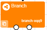
In all instances below key will be replaced in your data by the actual key of that node, which you can find in the Experiment Tree. For example, in the image below, the key for this Branch node would be 'oqq9'.

Questionnaire Builder 2 columns (long-format)

This is for long-format data only. Every questionnaire data file will also include the experiment information columns shown above.

Questionnaire Builder 2 columns (short-format)

This is for short-format data only. Every questionnaire data file will also include the experiment information columns shown above.

In all instances below the X will be replaced with the actual object ID number of the relevant component in your questionnaire. You can find the object ID within the Questionnaire Builder at the top-right of the component settings. In the below example, the object ID is '6'.

Task Builder 2 columns

Every task data file will also include the experiment information columns shown in the table at the top of this page.

Legacy tooling

Questionnaire Builder 1 columns (long-format)

Every questionnaire data file will also include the experiment information columns shown in the table at the top of this page.

Questionnaire Builder 1 columns (short-format)

Task Builder 1 columns

Time on Task

For each participant for each node, you will get additional rows to mark when participants BEGIN and END the task. This row can be identified because the value in the Response column will be BEGIN or END.

These rows will come with timestamps. Additionally, in the END row you will also get a reaction time in the Reaction Time column that is the time since the BEGIN timestamp. This can be used to calculate the time taken to complete the task.

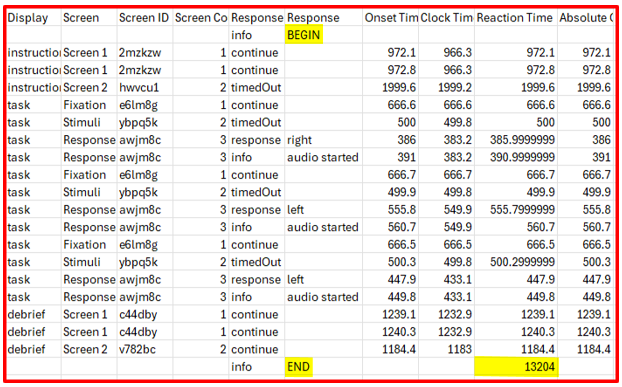
The above explanation applies to data collected from Task Builder 2, Game Builder and Shop Builder. For Questionnaire Builder 2, the metric will be recorded to the Tag column in the data output instead.

From Gorilla to Tidy Data

One of our users, Dr Emma James, has put together a step-by-step guide to data processing using the tidyverse package with RStudio.

This tutorial shows you how to set up the tidyverse in RStudio, read in your data, filter out anything you don't need, and calculate averages.

It also explains how to deal with more than one experimental condition, combining output files, and reshaping your dataset!

The tutorial can be found on Emma's site.

R Overview

R is a programming language that many researchers use for transforming and manipulating data. It is also used to perform statistical analyses.

RStudio is what's known as an Integrated Development Environment (IDE), which just means that you can use the RStudio programme to write and edit code in R.

This walkthrough will get you started with R and RStudio so that you can use it to transform your Gorilla data files ready for statistical analysis.

Downloading and Installing R

R:

1. Go to www.r-project.org
2. Click the download R link under the “Getting Started” header.
3. Select a mirror - you want to pick one that's relatively close to your location.
4. Depending on your operating system, click on the Download R for Windows/Download R for Linux/Download R for (Mac) OS X link at the top of the page.
5. Click the base link at the top of the page.
6. Click the Download R [version number] link at the top of the page.
7. Follow the installation instructions.

Downloading and Installing RStudio

RStudio:

1. Go to www.rstudio.org
2. Click on the Download link underneath the 'RStudio' image.
3. Scroll to the bottom of the page and select the appropriate installer for your system.
4. Follow the installation instructions.

Opening a New Script in R

When you open Rstudio, you will see a box on the left called Console, a box in the upper right with Environment and History, and a box in the lower right with Files, Plots, Packages and Help. To input commands easily, you will need to open a fourth box, called a Script.

A script is like a document in which you can write and save code. The code in your script can be run easily and repeatedly. You can also copy and paste code from others into your own script, and export your script as a .R file so others can use it.

To open a new script, press the Open New icon in the top left hand corner, then select R Script.

This is your new script. You can write your code or copy and paste code from others into here.

Getting started with R

The script below allows you to get started with your Gorilla data in R. It explains how to import your file and how to tidy the data.

This is important, as sometimes, when you download the available CSV data from your experiment, there is a lot of files with a lot of data - which can be overwhelming!

Adding the script below to R makes it easy to start analysing your data by tidying it and making it more manageable.

To use the script below, copy and paste everything in the box into the top left-hand section of your new RStudio script. Then follow the instructions written in the comments of the script itself (comments begin with a “#”).

# This is a package that is used throughout our R scripts
# If this is your first time using R or this package, you will have to remove the hashtag on the line below to turn it from a comment into code and install the package
# install.packages("tidyverse")
library(tidyverse)

################# Looking at one task/questionnaire #################
# This is a script to use to explore and tidy your data from a single task or questionnaire
# Set your working directory to the folder in which all your CSV files are located
setwd("C:/User/Folder/Subfolder")

# Read in your task or questionnaire
task <- read_csv("data_exp_1111-v1_task-1111.csv")
questionnaire <- read_csv("data_exp_1111-v1_task-1111.csv")

# To see all your data in a separate tab
View(task)
View(questionnaire)

################# Filtering rows #################
# The data produced has many rows, and not all the information may be relevant
# If we know that all the information we need for analysis occurs in a specific component type, e.g. a response component, we can specifically select those rows to minimise the size of the dataset
# The task below filters by the column 'Component Name' and only keeps rows with a "Keyboard Response" component, but you can specify any row in your dataset
task <- task %>%
  filter(`Component Name` == "Keyboard Response")
# The questionnaire example here filters long-format data by responses only (and excludes actions) and where the `Object Name` was either one of two possibilities, but you can specify any row in your dataset.
questionnaire <- questionnaire %>%
  filter(`Response Type` == "response" &
         (`Object Name` == "important-1" | `Object Name` == "important-2"))

################# Selecting columns #################
# Gorilla provides a lot of information, and depending on your task/questionnaire, not everything may be relevant
# This will show you the names of all the headers in your d dataset, so you can choose the ones you wish to keep
names(task)
# The lines below will select the key variables you specify
task <- task %>%
  select(`Participant Private ID`,
         `UTC Date`,
         `Component Name`,
         Response,
         `Spreadsheet: Answer`,
         `Reaction Time`)
# The example here selects these specific columns to focus on, however, this will depend on your hypothesis

# You can also rename your column names if you want (but this also works within the select() function above!)
task <- task %>% 
  rename(ID = `Participant Private ID`,
         date = `UTC Date`,
         component = `Component Name`,
         response = Response,
         answer = `Spreadsheet: Answer`,
         RT = `Reaction Time`)

Pressing CTRL+ENTER will run the line of code you are currently on and move you to the next line. Making your way through the code using CTRL+ENTER will allow you to see how the dataset gradually takes shape after every line of code – this is also a good way of easily spotting any errors if you encounter them whilst running the script.

CTRL+ENTER will also run any highlighted code, so if you want to run the whole script together, highlight it all and press CTRL (or Command ⌘ on a Mac) +ENTER You can also press CTRL (or Command ⌘ on a Mac) +ALT+R to run the entire script without highlighting anything

We are constantly updating our R support pages. For more information about Gorilla metrics specifically please consult our support page which contains guides on metrics.

Combining Files in R

Adding the Script below to R makes it easy to combine CSV files containing your task or questionnaire data into a single CSV file. The CSV will be formatted so that the final row of one CSV is followed by the first row of the next CSV.

The script below is divided into two parts, based on the CSV files you want to combine. If you want to combine questionnaires or identical tasks (that are separated due to the experiment tree, e.g. randomiser node) the first part of the script will explain how to do this.

Combining CSV files of different tasks is a bit more complicated, due to the nature of the complexity of the task builder, so the second part of the script addresses how to combine such CSV files.

Combining CSVs of questionnaires or identical tasks:

# install.packages("tidyverse")
library(tidyverse)

# Set your working directory to the folder in which all your CSV files are located
setwd("C:/User/Folder/Subfolder")

################# Combining CSVs- Questionnaires/Same tasks #################
# This is the script to use if you want to combine questionnaires or identical tasks (differing only e.g. on counterbalancing)
# You list the files you want to combine, each with a "" around them
files <- c("data_exp_1111-v1_task-1111.csv",
           "data_exp_2222-v2_task-2222.csv")
# files <- c("data_exp_1111-v1_questionnaire-1111.csv",
#            "data_exp_2222-v2_questionnaire-2222.csv")

# You can combine the CSVs using either base R or tidyverse (subject to preference)
# using tidyverse
combined_data <- lapply(files, read_csv) %>% 
  bind_rows()
# using base R
combined_data <- do.call("rbind", lapply(files, read_csv))

# Your dataset also has some rows that contain "END OF FILE" and nothing else. You can exclude these rows using this line.
# using base R
combined_data <- combined_data[combined_data$`Event Index` != "END OF FILE",]
# using tidyverse
combined_data <- combined_data %>%
  filter(`Event Index` != "END OF FILE")

# This line exports your combined data as a CSV. This new CSV will be called "combined_data.csv" and will appear in your working directory
write_csv(combined_data,"combined_data.csv")

Combining CSVs of different tasks and questionnaires:

# install.packages("tidyverse")
library(tidyverse)

# Set your working directory to the folder in which all your CSV files are located
setwd("C:/User/Folder/Subfolder")

################# Combining CSVs - Different tasks/questionnaires #################
# To combine tasks that are different, this will require sequential going through the tasks and adding the relevant data from each
# Firstly, you import a task or questionnaire that will contain your base information (information you want to be present in the final dataset)
# In this example, I have 3 tasks that I want to combine
task1 = read_csv("data_exp_1111-v11_task-1111.csv")
task2 = read_csv("data_exp_2222-v22_task-2222.csv")
task3 = read_csv("data_exp_3333-v33_task-3333.csv")

# I choose my first task as the base and create a new dataset 'final'
final <- task1 %>%
  filter(`Component Name` == "Keyboard Response") %>%
  mutate(task = "task1") %>%
  select(`Participant Private ID`,
         `Participant OS`,
         `Participant Device`,
         `UTC Date`,
         `Spreadsheet: Answer`,
         Response,
         `Reaction Time`)

# Now, I take my second task and choose the specific columns I am interested in
task2 <- task2 %>%
  filter(`Component Name` == "Text Entry") %>%
  select(`Participant Private ID`,
         `Spreadsheet: Answer`,
         Response,
         `Reaction Time`)

# I do the same with my third task
task3 <- task3 %>%
  filter(`Component Name` == "Keyboard Response") %>%
  select(`Participant Private ID`,
         `Spreadsheet: Answer`,
         Response,
         `Reaction Time`)

# Next we can combine both tasks with our base, and then use grouping and filling to copy over the OS, Device, and Date information to the rest of that participant's data
final <- final %>% 
  full_join(task2) %>%
  full_join(task3) %>%
  group_by(`Participant Private ID`) %>%
  fill(`Participant OS`,
       `Participant Device`,
       `UTC Date`)

# I can then save a new .csv file with this data onto my hard drive
write_csv(final,"final_combined.csv")

Now you should have a new CSV in the folder you specified as your working directory called “combined_data.csv” or "final_combined". This contains all the data from your separate CSVs.

Long-to-Short Data Transformation using R

To use the script below, copy and paste everything in the box into the top left-hand section of your new RStudio script. Then follow the instructions written in the comments of the script itself (comments begin with a ‘#’).

The scripts below show how to transform your task data from long- to short-format data with some basic data processing. You shouldn't need to do this with your questionnaire data because you can choose to have the questionnaire files in long- or short-format when you download your data!

Task: long to short data transformation

# install.packages("tidyverse")
library(tidyverse)

# Set your working directory to the folder in which all your CSV files are located
setwd("C:/User/Folder/Subfolder")

# This is a script to use to transform your data from long to short
# We'll also do some basic processing of RTs and accuracy for two different experimental conditions based on meta-data in the spreadsheet

task <- read_csv("data_exp_1111-v1_task-1111.csv")

# This filters the data so that we only have the rows where a response was required
# And it only selects the four main columns of interest
task <- task %>%
  filter(Screen == "Stimuli") %>%
  select(`Participant Private ID`,
         `Spreadsheet: Condition`,
         `Correct`,
         `Reaction Time`) %>%
  group_by(`Participant Private ID`,
           `Spreadsheet: Condition`) %>%
  # Calculates the mean RT and the proportion correct
  summarise(mean_RT = mean(`Reaction Time`),
            accuracy = sum(Correct)/length(Correct))

# Next we create new column names by combining the spreadsheet metadata about conditions
# with the names of the current mean_RT and accuracy columns
# It will then populate each column with the values specified
task_short <- task %>%
  pivot_wider(id_cols = `Participant Private ID`,
              names_from = `Spreadsheet: Condition`,
              values_from = c(`mean_RT`, accuracy))

# Now we have one row per participant with five columns:
# 1) Participant Private ID
# 2) mean_rt_[conditionA]
# 3) mean_rt_[conditionB]
# 4) accuracy_[conditionA]
# 5) accuracy_[ConditionB]

# Export as csv
write_csv(task_short, "Task_Short_Format.csv")

Now you should have a new CSV in the folder you specified as your working directory called "Task_Short_Format.csv” with accuracy as a proportion and the mean RT in milliseconds for each experimental condition, and each participant should only take up one row of data.

Worked Examples of R analysis

We cover plenty of worked examples of data analysis using R in our Gorilla Academy!

Browse through the lectures and video walkthroughs on the Gorilla Academy page.

Excel Overview

Excel can be used to transform and clean your data.

This walkthrough will show you how you can use Excel to filter and clean your data, allowing you to choose only the information you may need.

It also highlights how Excel's pivot tables can be used to get your data in the format you want.

It's worth mentioning that pretty much anything you can do here in Excel can also be done in Google Sheets or open source spreadsheet software.

Clean and Filter Your Data using Excel

The raw CSV file you download from Gorilla contains a lot of information that you probably won't need. We want to give you a complete picture of your participant data, so if you happen to be interested in e.g. the local time when a participant completed your experiment, that information is available to you. However, you are probably only going to be interested in a few specific metrics.

The video below will walk you through what the different columns in your data file are, and how you can filter your data to view the information you need.

NB: The below video was made using data from the Legacy Tool Task Builder 1. The information contained is still accurate, but some of the column names will be a little different. For example, you'll no longer see the columns 'Zone Name' or 'Zone Type' because Task Builder 2 doesn't use zones. In Task Builder 2 data you'll find the same sort of information in the 'Object Name', 'Component Name', and 'Response Type' columns instead.

Length (mins): 2:50

You can also use Excel's filtering function to get rid of rows you don't need in your data. In this example, we are working with questionnaire data, but we are not interested in any ‘quantised’ data. Therefore, we want to remove all data rows which are of the form ‘quantised’ from our questionnaire data. Here’s how to do this in 10 quick steps!

1. Open your Gorilla metrics file in Excel. It will look something like this:

2. Navigate to the Data tab:

3. Click somewhere within the data, then click on the Filter button:

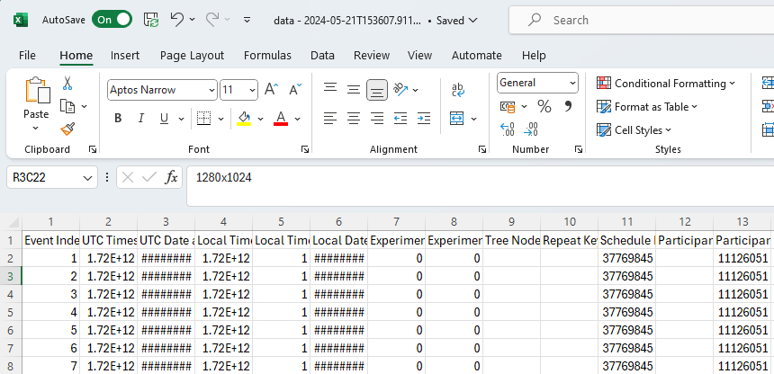
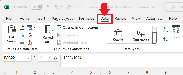
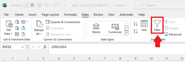
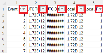
You will now see mini arrows (filter arrows) at the top of all your columns like this:

4. Navigate to the column which contains the information that identifies the data you want to remove. The column that identifies whether data is quantised or not is the 'Key' column. (If you used Questionnaire Builder 1 to collect your data, the relevant column will be called 'Question Key'.)

5. Click the filter arrow for the Key column:

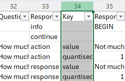
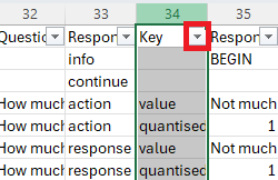
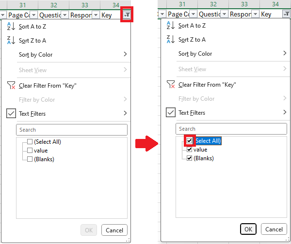
This will bring up a menu which looks something like this:

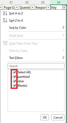
Notice all the ticks in the boxes? At the moment, all our data is selected and is being displayed.

6. Uncheck the '(Select All)' box (this will deselect all filters).

7. Next check only the data we want to remove and press 'OK'. i.e. select 'quantised'. (In Questionnaire Builder 1, you will have to select every box that corresponds to quantised data - these will be in the form 'questionkey-quantised'.) Your filter box should now look something like this:

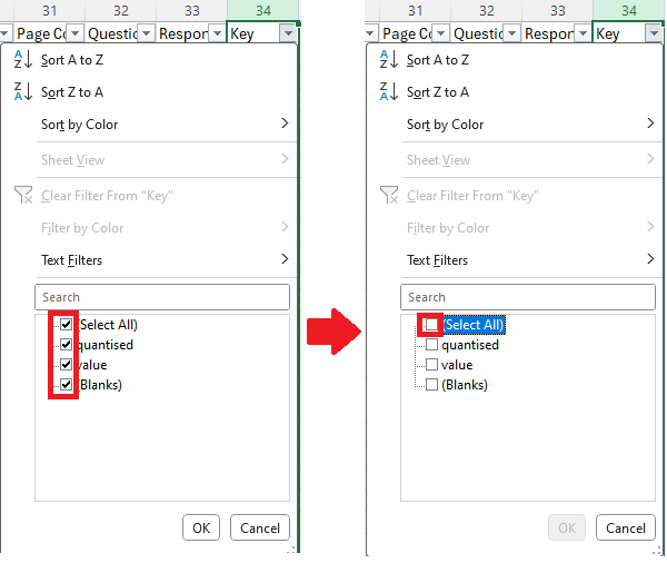
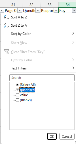
Your data spreadsheet will now look something like this:

Notice how only the quantised data is being displayed on your spreadsheet. (In this example there are only two rows; you will likely have more participants and thus many more rows.)

8. Now highlight all the rows of data: Make sure you highlight the whole row by clicking on the row number itself. To quickly select all rows, first click the top row of data, then hold the SHIFT key ( on your keyboard) and press the last row of data. This will select all the rows between the two points.

9. Now while keeping the rows selected, right-click on the any of the row numbers and select 'Delete Row' from the menu.

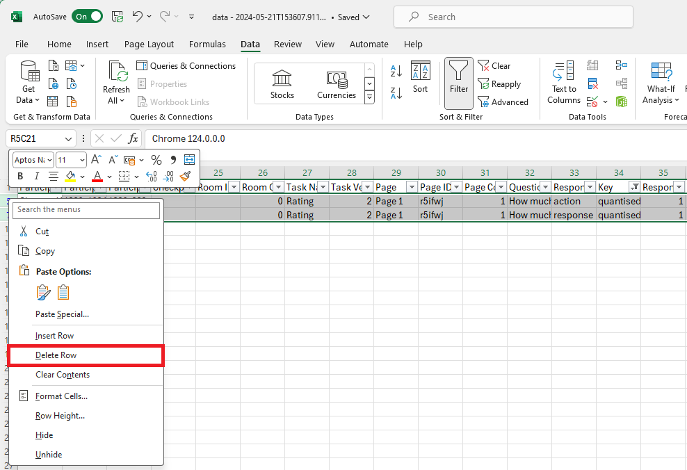
You should now be left with a seemingly blank looking data sheet:

10. Finally, remove all the filters and we have our cleaned questionnaire data! Click again on the 'Key' filter arrow, check '(Select All)', and press OK:

Your data sheet will now look like this:

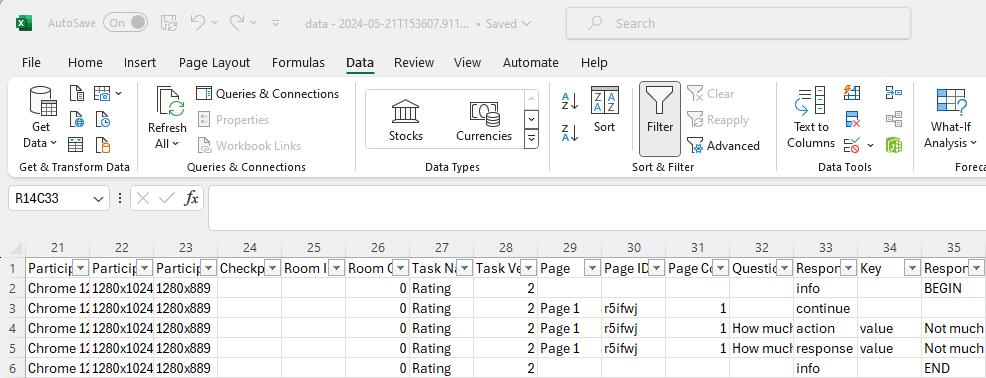
Your data no longer contains any ‘quantised’ data rows!

Excel Pivot Tables

If you're not familiar with Pivot Tables, get ready to revolutionise the way you edit your data! Pivot Tables are an incredibly useful way to get your data into the format you want it in. For instance, you can ask Excel to calculate the mean of each participant's score over a series of trials, and enter those means into a new table where each participant has one row.

Learn the basics of Pivot Tables for transforming task data from long to short format in the video below!

NB: The below video was made using data from the Legacy Tool Task Builder 1. The information contained is still accurate, but some of the column names will be a little different. For example, you'll no longer see the columns 'Zone Name' or 'Zone Type' because Task Builder 2 doesn't use zones. In Task Builder 2 data you'll find the same sort of information in the 'Object Name', 'Component Name', and 'Response Type' columns instead.

Length (mins): 4:18

Combining Data

Learn how to combine metrics from two datasets into one Excel file in the video below!

If you are planning to use SPSS for your data analysis, have a look at their guide to merging files for SPSS-ready data.

NB: The below video was made using data from the Legacy Tool Task Builder 1. The information contained is still accurate, but some of the column names will be a little different. For example, you'll no longer see the columns 'Zone Name' or 'Zone Type' because Task Builder 2 doesn't use zones. In Task Builder 2 data you'll find the same sort of information in the 'Object Name', 'Component Name', and 'Response Type' columns instead.

Length (mins): 3:29

Advanced Data Handling in Excel - Pivot Tables and Text Responses

One downside of pivot tables is that they don't allow you to pivot text responses. However, this is are ways to get around this using Excel functions. We'll take you through a couple of ways this could be achieved, including a nifty solution using the INDEX and MATCH functions, just like we used in the previous 'Combining Data' video. Watch the video below to find out how to emulate pivot tables this way!

NB: The below video was made using data from the Legacy Tool Questionnaire Builder 1. The information contained is still accurate, but some of the column names will be a little different. For example, you'll no longer see the column 'Question Key'. In Questionnaire Builder 2 data you'll instead find similar information in the 'Object ID' and 'Key' columns.

Length (mins): 9:27

Worked Example of data preprocessing

You can find worked example of data preprocessing using Excel in our Gorilla Academy!

See our lecture on organising data in Excel to learn about Excel formulas to calculate new variables and creating pivot tables to prepare your data for analysis!

Mousetracking Data to Plots in R

This guide contains code for converting Gorilla mouse-tracking data to mousetrap format and using mousetrap() functions to create plots.

To use the script below, copy and paste all of it into the top left-hand section of your new RStudio script. Then follow the instructions written in the comments of the script itself (comments begin with a “#”).

#Mouse tracking in Gorilla gives two types of dataset: response data and mouse-tracking data. 
#Response data are the normal Gorilla task data, showing what screens participants saw, how many answers they got correct etc.
#Mouse-tracking data present coordinates for zones and mouse movements within an individual trial. 
#There should be one response dataset in total, and one mouse-tracking dataset for each trial in the experiment.

#Before you start the guide below, make sure that all the individual mouse-tracking files (in xlsx format) are together in 
#the same folder with no other unrelated xlsx files.

#Note: the latest version of mousetrap at time of writing is v3.1.2.

############################## 1) Load all the packages you will need. ##############################
#library() loads packages. You need to install packages before you can load them. If you do not have any of the packages
#listed below installed, run the install.packages line below for each of the packages listed. 
#install.packages("mousetrap")
library(mousetrap)
library(readxl)
library(data.table)
library(dplyr)
library(ggplot2)

############################## 2) Import all the Gorilla mouse-tracking data into R. ##############################
#Here is an example way of importing all your mouse-tracking excel files into R. You can use other ways if you want to, as 
#long as they end up with a single data frame containing all the mouse-tracking data together.
#Set your working directory as the folder in which you have saved your data files. This tells R where to look for files.
setwd("C:/Users/Adam Flitton/Desktop/mousetracking")

#Create a list of the xlsx files in your working directory.
xslxfiles<-list.files(pattern="*.xlsx")

#Import all the excel files in the list.
xlsx.df.list<-lapply(xslxfiles,read_excel)

#Combine all these imported excel files into a single data frame. 
gorilla.traj<-rbindlist(xlsx.df.list)

############################## 3) Prepare the data for importing as an mousetrap object. ##############################
#Drop all the rows that contain coordinates for the zones. In these rows there is no mouse tracking data, so we do not need
#them for now.
gorilla.traj<-gorilla.traj[gorilla.traj$type=="mouse",]

#Gorilla data gives you normalised coordinates as well as raw ones. We can only import raw or normalised at the same time.
#Let's drop the normalised ones so we can just import the raw data.
gorilla.traj<-within(gorilla.traj,rm(x_normalised,y_normalised))

############################## 4) Use mousetrap's import function to write in the Gorilla data. ##############################
#This function requires you to specify columns in your dataset including x, y and timestamps. 
#It also requires a column in your dataset that shows the different trials (argument "mt_id_label"). 
#row_index should cover this in most datasets, as it prints what row of the spreadsheet the participant is on, which is more
#often than not a new trial.
#If you have a different trial column, replace "row_index" with whatever this column is called in the code below. 
gorilla.mt<-mt_import_long(gorilla.traj,xpos_label="x",ypos_label="y",timestamps_label="time_stamp",
                           mt_id_label="row_index")

#Now you have your mousetrap data object! It's a list containing two data frames:
gorilla.mt[["trajectories"]] 
#This contains your coordinates data in mousetrap format. The rows in this dataset are specified by the mt_id_label above.
gorilla.mt[["data"]] 
#This is basically empty at the moment, containing a row for each trial without much else. It isn't necessary
#to have much data in this data frame to use many of the functions in mousetrap (we will add a column to it later that 
#shows what condition the trial is in as this helps with plotting different conditions)

############################## 5) Use mousetrap's measures function to get summary statistics. ##############################
gorilla.mt<-mt_measures(gorilla.mt, use = "trajectories",save_as="measures",
                        dimensions = c("xpos", "ypos"), timestamps = "timestamps",
                        verbose = FALSE)

#This adds another data frame to your mousetrap list called "measures" that contains useful summary statistics. 
View(gorilla.mt[["measures"]])

############################## 6) Optional: conditions. ##############################
#If your study does not have conditions or anything else that you want to break the results down by, move on to the next step. 
#Below is one way of adding in conditions to your mouse-tracking dataset. This way works if you have a column in your Gorilla
#response dataset that shows what conditions participants are in. This might be a metadata column, for instance.
#This way also assumes that the Trial Number column in your Gorilla response dataset corresponds to different trials, just 
#like row_index does for the mouse-tracking data. 

#It may be that your data are in a different format. If so, see step 9 for an alternative (more manual) way of adding conditions.

#First, import the Gorilla response data. In this example this excel file is in the same working directory as before (as it is
#a CSV rather than an xlsx, it wasn't lumped in with the mouse-tracking data earlier). It may be that your response data are
#in a different place, in which case change your working directory again (remove the hash from the line below and change its path)
#before you read in the data.
#setwd("C:/Users/Adam Flitton/Desktop/mousetracking/PLACE WHERE RESPONSE DATA ARE")
gorilla.response.data<-read.csv("BetaZoneMouseTrackingData.csv",na.strings=c("","NA"))

#Stratify these data to only include rows in which a participant made an attempt. These rows are the response rows that give
#information about what answer they gave, how long it took them, whether it was correct etc. Other rows (that this function
#removes) just provide links to the mouse-tracking datasets and show fixations/continuation screens. 
gorilla.response.attempts<-gorilla.response.data[gorilla.response.data$Attempt %in% 1,]

#Now we have a dataset that shows what condition the different trials were in. In this example, the column with the condition
#information is called "Metadata" and the column with the trial information is called "Trial.Number". 
#We need to take this condition information and add it to our mousetrap data, making sure to match up the trials. 
#In the mousetrap dataset, trial number is shown in the column "row_index". So we need to make sure that we match up "Trial.
#.Number" with "row_index".
#Remember: if you used a column that is not "row_index" to specify trials when you imported your data above, use the name of
#this column instead of "row_index" in all of the code below.
#The code below creates a new column in our mousetrap object called "condition" and populates it with the entries in the 
#"Metadata" column mentioned above, matching by "row_index" and "Trial.Number".

gorilla.mt[["data"]]$condition<-
  gorilla.response.attempts$Metadata[match(gorilla.mt[["data"]]$row_index,gorilla.response.attempts$Trial.Number)]

#You can add any column from your response dataset using this same matching. Below makes a different column called "Correct"
#then populates the column with whether a response was correct from the "Correct" column (rather than the "Metadata" column). 
#gorilla.mt[["data"]]$Correct<-
#gorilla.response.attempts$Correct[match(gorilla.mt[["data"]]$row_index,gorilla.response.attempts$Trial.Number)]

#Note: you can also use the above to break data down by any other group, such as participant. Just use the column that
#distinguishes between participants instead of the column that distinguishes between conditions. 

############################## 7) Optional: rectangles for graphs. ##############################
#In the step after this one you will make some graphs from the data. It might be that you want to present rectangles on this
#graph that show where the buttons and stimuli were on the screen. If you don't want to do this, move on to the next step.

#Create a copy of the original unaltered mouse-tracking dataset that contains zone names. 
gorilla.traj.rectangles<-rbindlist(xlsx.df.list)

#Create a matrix from the zone coordinates in the mouse-tracking dataset. 
#Make a variable containing the names of the zones that you want to represent with rectangles on the graph.
#The zones presented to participants in the task are listed in the "zone_name" column of the mouse-tracking dataset. In this
#example I assume that the rectangles that will be presented on the graph correspond to the zones called "Stimulus", 
#"ButtonLeft", and "ButtonRight" in the data. You can change these names in the row below to be whatever you have called them. 
matrix.contents<-c("Stimulus","ButtonLeft","ButtonRight")

#Now extract the zone_x, zone_y, zone_width and zone_height values for the zones listed in the matrix.contents variable
#specified above.
matrix.data<-filter(gorilla.traj.rectangles, zone_name %in% matrix.contents)
matrix.data<-matrix.data[1:length(matrix.contents),c("zone_x","zone_y","zone_width","zone_height")]

#Put these data in a matrix that will be referred to in the plot function later. 
rectangles<-as.matrix(sapply(matrix.data, as.numeric)) 
rectangles<-unname(rectangles)

############################## 8) Use mousetrap's plot functions. ##############################
#a) All the mouse-tracking data together:
mt_plot(gorilla.mt,use="trajectories",use2="data",x="xpos",y="ypos")
#b) Colour the lines by the trial number:
mt_plot(gorilla.mt,use="trajectories",use2="data",x="xpos",y="ypos",color="row_index")
#c) Colour the lines by condition:
mt_plot(gorilla.mt,use="trajectories",use2="data",x="xpos",y="ypos",color="condition")
#d) Add points:
mt_plot(gorilla.mt,use="trajectories",use2="data",x="xpos",y="ypos",points=TRUE,color="condition")
#e) Add rectangles:
mt_plot(gorilla.mt,use="trajectories",use2="data",x="xpos",y="ypos",points=TRUE,color="condition")+
  mt_plot_add_rect(rect=rectangles)
#f) You can customise the rectangles in the same way that you would customise a geom_rect in ggplot:
mt_plot(gorilla.mt,use="trajectories",use2="data",x="xpos",y="ypos",points=TRUE,color="condition")+
  mt_plot_add_rect(rect=rectangles,color="NA",fill="blue",alpha=0.2)
#g) You can add themes and axis labels just like any other ggplot:
mt_plot(gorilla.mt,use="trajectories",use2="data",x="xpos",y="ypos",points=TRUE,color="condition")+
  mt_plot_add_rect(rect=rectangles,color="NA",fill="blue",alpha=0.2)+
  xlab("X axis position")+
  ylab("Y axis position")+
  theme_classic()
#h) If you add the argument "only_ggplot=TRUE", the plot will be blank, but you can add paths and points to it like you
#would for a normal ggplot, which lets you customise them.
mt_plot(gorilla.mt,use="trajectories",use2="data",x="xpos",y="ypos",color="condition",only_ggplot=TRUE)+
  mt_plot_add_rect(rect=rectangles,color="NA",fill="blue",alpha=0.2)+
  geom_path(size=1)+
  geom_point()+
  scale_color_manual(values=c("Congruent"="purple","Incongruent"="green"))+
  theme_classic()

############################## 9) Alternative way of adding conditions. ##############################
#A more manual way of adding conditions might be needed for certain data structures. Below replaces step 2 in the above guide. 
#This way works by importing the data files for the different conditions as separate datasets at the beginning, and manually
#adding a column to each of these condition-specific datasets that states which condition they are.
#So this code assumes that you have separate folders, each one containing all the xlsx files for an individual condition.

#Import all the data from these folders separately so we have two separate datasets in R, one for each condition.
setwd("C:/Users/Adam Flitton/Desktop/mousetracking/condition1")
xslxfiles.cond1<-list.files(pattern="*.xlsx")
xlsx.df.list.cond1<-lapply(xslxfiles.cond1,read_excel)
cond1<-rbindlist(xlsx.df.list.cond1)

setwd("C:/Users/Adam Flitton/Desktop/mousetracking/condition2")
xslxfiles.cond2<-list.files(pattern="*.xlsx")
xlsx.df.list.cond2<-lapply(xslxfiles.cond2,read_excel)
cond2<-rbindlist(xlsx.df.list.cond2)

#Add a column called "condition" to each of these separate datasets, and fill this column with a label showing which condition each
#dataset is. 
cond1$condition<-"Congruent"
cond2$condition<-"Incongruent"

#Then combine these datasets together. 
gorilla.traj<-rbind(cond1,cond2)

#Now in the guide above continue onto step 3 and skip step 6.

Pressing CTRL+ENTER will run the line of code you are currently on and move you onto the next line. Making your way through the code using CTRL+ENTER will allow you to see how the dataset gradually takes shape after every line of code. CTRL+ENTER will also run any highlighted code, so if you want to run the whole script together, highlight it all and press CTRL+ENTER. You can also press CTRL+ALT+R to run the entire script without highlighting anything.

We will be adding more guides for data transformation using R soon. For more information about Gorilla please consult our support page which contains guides on metrics.

Analysis of Eye Tracking Data using R

For more information on how to analyse eye tracking data in R with Task Builder 1, visit our TB1 eye tracking pages.

While we do not currently offer specific guidance on how to analyse eye tracking data in R with Task Builder 2, you can find general information about the structure of the data and tips for analysis in our TB2 eye tracking guide.